This project demonstrates various algorithms for robot motion planning, including RRT (Rapidly-exploring Random Trees) with A*, Visibility Graph with Dijkstra, and Approximate Cell Decomposition. The implementation is carried out in MATLAB, and each method is applied to different environments and obstacle configurations. The project aims to navigate a robot from an initial position to a goal while avoiding obstacles in a 2D workspace.

Features

  • RRT with A*: Combines RRT for map generation and A* for finding the optimal path. Two versions of the RRT are implemented:
    • RRT Tree: Uses a tree structure for connecting nodes and building paths.
    • RRT Graph: Uses a graph structure, allowing for more complex connections between nodes.
  • Visibility Graph with Dijkstra: Implements both the standard Dijkstra method and a heuristic variation for pathfinding.
  • Approximate Cell Decomposition: Breaks the map into grid cells and calculates shortest paths using Dijkstra. It also considers robot orientation.

MATLAB Environment Generating

To create an environment that follows the constraints of the project I created a ‘createRandomEnvironment.m’ file. In addition to the number of obstacles, my ‘CreateEnvironment.m’ file has two other inputs, aSize and bSizeRatio.

aSize represents the size of the robot you want to generate and bSizeRatio is the numerator for the scalar value used in B generation. The randomly generated obstacle can be any size between 1 and the bSizeRatio as well as have 3 to the maxObsSide number of sides. This allows for the random environment to have more unique obstacle shapes and sizes. CreateEnvironment outputs the following arguments to be used in the methods bellow.

  • A: a 2xN array containing x and y coordinates of the robot’s vertices relative to a body fixed reference frame located at [0, 0]. The robot is represented as a red polygon.
  • B: a 1xM cell array whose elements represent individual obstacles within a world frame located at [0, 0]. Obstacles are represented as a blue polygon.
    • B{i} – a 2xK array containing x and y coordinates of the ith obstacle’s vertices relative to a world frame located at [0, 0].
  • q_init: a 3×1 array containing the initial position and orientation of the robot.
  • q_goal: a 3×1 array containing the goal position and orientation of the robot. – bounds: 2×4 bounding points of map (rectangular shape)

In addition, the configuration space of the obstacles (shown in green or light green) are generated in software and shown around each obstacle as CB.

In addition to this, there are saved environments in the Environments folder that can be used at any time

Method III – Approximate Cell Decomposition with Dijkstra

Method 3 uses the Approximate Cell Decomposition method to generate the map of the workspace. To consider both position and orientation, CBi of Bi is generated by calculating all the obstacle spaces using every robot possible orientation. You can see the layers of CBs around each obstacle in the Figure below.

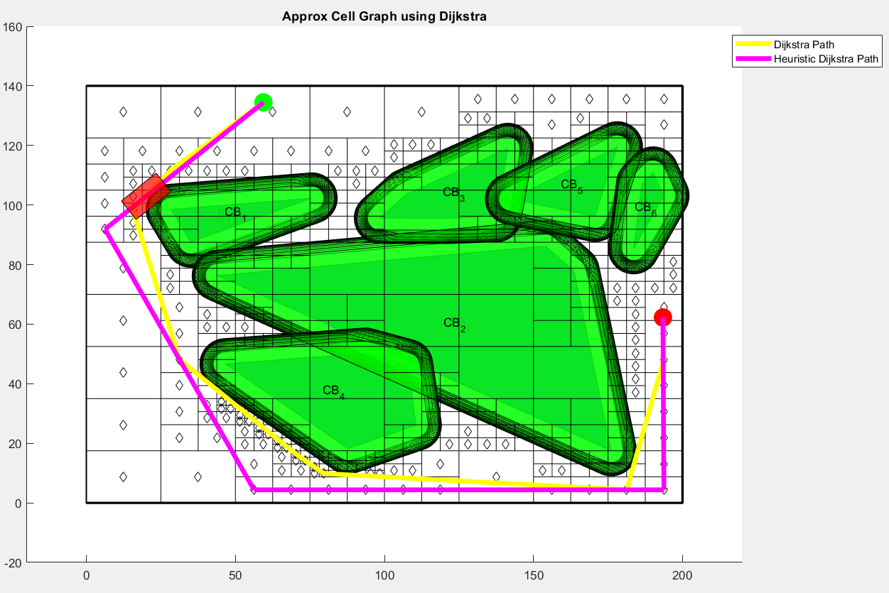
Then using Approximate Cell Decomposition, the map is broken down into grids that show if a space is occupied or free. Using the adjacency matrix generated from the decomposition of the workspace, the new Dijkstra algorithm is applied to find the shortest path from initial position to goal.

For each part of the path the orientation is calculated using the ‘atan2’ function. This function will find the angle between the robot’s current orientation and the paths. Using this function also keeps the angle between pi and -pi allowing the rotation to be directional and short.

Lastly, the robot is animate along the planned path using differential drive mechanics and orientation. The robot considers omega the rotational velocity when rotating at robots’ position. Then after aligning with the next path the robot moves forward, translating the position based on the velocity. All speeds are calculated using the time step. The rotation was acting weird, so I had to remove the omega portion.

.

Method II – Visibility Graph with Dijkstra

Method 2 uses a Visibility Graph to demonstrate how different distance calculations can affect the outcome of a path.  The yellow solid line is the calculated path using the common Dijkstra path finding method we did together in class. The magenta line is the output path if a heuristic calculation was used in Dijkstra instead, like in A*. 

In addition to comparing the modification of Dijkstra, the Visibility Graph function also had some modifications. The previous Visibility Graph did not consider if the obstacle configuration spaces were overlapping. If the configuration space edges overlap with another it can not be considered in the Visibility Graph. .

Method I -RRT with A*

Method 1 incorporates A* logic to find the optimal path on a map which is generated using an RRT (Rapidly-exploring random trees) method. For this project I created two RRT programs, RRT Tree and RRT Graph. Both follow the same principle of a common RRT method, randomly generate points/nodes and connect said node to the closest node(s), checking each connection to make sure it does not fall within an obstacle. However, each program uses a different data structure to store nodes and find edges.

RRT Tree uses a tree structure to connect nodes via edges. Because a tree structure has a parent-child relationship between nodes, each node can only have one parent which results in a simple, treelike structure throughout the map. 

RRT Graph uses a graph structure to create a collection of nodes connected by edges. Unlike the tree structure, each node in the graph can have multiple parents or none. This adds more complexity to the algorithm, so the RRT Graph follows a slightly different structure. The RRT Tree structure generates a node and creates the correlation edges, but the RRT Graph structure generates all the random nodes first, then once all the nodes are populated, it will iterate through each node connecting it to other nodes within a predetermined distance from it.

Both the RRT Tree and RRT Graph algorithms are implemented using the same script, Method1.m. After generating the map, the Astar_CustomG.m function is used to find a path, if one exists, between the start node q_init and the goal node q_goal.